
Analytical Functions and Their Usage
Analytical functions are powerful SQL tools that enable complex calculations while preserving row-level detail. They shine in scenarios requiring:
- Rankings and percentiles (top N per group, quartiles)
- Moving calculations (averages, sums)
- Period-over-period comparisons (monthly growth)
- Sessionization and sequence analysis
- Relative calculations (differences from averages)
The key advantage is performing these operations in a single pass through the data while maintaining access to all row details. They eliminate the need for many self-joins and correlated subqueries that were traditionally used for such calculations.
Master SQL Analytical Functions Interview Questions and Answers
Proper use of window functions can make queries both more readable and more efficient. However, they work best when you understand the window frame specifications and partition carefully to avoid excessive memory usage. For large datasets, pay special attention to the ORDER BY clauses in your OVER() specifications, as these often require sorting operations that can be expensive.
Real-world applications include financial analysis (running balances), operational metrics (rolling averages), customer behavior analysis (session grouping), and performance benchmarking (department rankings). Mastering window functions can elevate your SQL from simple data retrieval to sophisticated analytical processing.
Q1. What are analytical/window functions in SQL and how do they differ from aggregate functions?
Analytical functions, also called window functions, perform calculations across a set of table rows related to the current row. Unlike aggregate functions that collapse multiple rows into a single result, window functions maintain individual rows while adding computed values.
The key difference is that aggregate functions (like SUM, COUNT, AVG) group data and return one result per group, while window functions can return multiple results – one for each row in the original dataset.
-- Aggregate function (collapses rows)
SELECT department, AVG(salary)
FROM employees
GROUP BY department;

-- Window function (preserves rows)
SELECT name, department, salary,
       AVG(salary) OVER(PARTITION BY department) as avg_dept_salary
FROM employees;
Q2. Explain the OVER() clause in analytical functions and its significance
The OVER() clause is what defines the “window” or set of rows that the analytical function operates on. It’s the heart of window functions, specifying how to partition and order the data before applying the function.
Without OVER(), functions like RANK() or AVG() wouldn’t know how to behave as window functions. The clause can be empty (OVER()) to operate on the entire result set, or contain PARTITION BY and ORDER BY specifications.
-- Simple OVER() using entire result set
SELECT name, salary,
       AVG(salary) OVER() as company_avg
FROM employees;

-- With PARTITION BY to create department windows
SELECT name, department, salary,
       AVG(salary) OVER(PARTITION BY department) as dept_avg
FROM employees;
Q3. What are the three main components of a window function syntax?
Window functions have three key parts:
- The function itself: Like RANK(), SUM(), LEAD(), etc.
- The OVER() clause: Defines the window frame
- Window specifications inside OVER():
- PARTITION BY (groups rows into partitions)
- ORDER BY (orders rows within partitions)
- Window frame (ROWS/RANGE between boundaries)
SELECT employee_id, department, salary,
       -- The three components:
       SUM(salary) OVER(                -- 1. Function
           PARTITION BY department      -- 2. Partition
           ORDER BY hire_date          -- 3. Order
           ROWS BETWEEN 1 PRECEDING    -- 4. Frame
               AND 1 FOLLOWING
       ) as moving_sum
FROM employees;
Q4. How do window functions differ from GROUP BY operations?
Window functions and GROUP BY both work with groups of data, but in fundamentally different ways:
- GROUP BY collapses each group into a single row in the output
- Window functions preserve all original rows while adding computed values
- With GROUP BY, you can only select grouped columns or aggregates
- With window functions, you can select all individual row data plus computed values
-- GROUP BY approach (loses individual row details)
SELECT department, COUNT(*) as emp_count
FROM employees
GROUP BY department;

-- Window function approach (keeps all rows)
SELECT name, department,
       COUNT(*) OVER(PARTITION BY department) as dept_count
FROM employees;
Q5. Explain the difference between ROW_NUMBER(), RANK(), and DENSE_RANK() with examples
These ranking functions all assign numbers to rows, but handle ties differently:
- ROW_NUMBER(): Always gives unique numbers (1,2,3), even for ties
- RANK(): Gives same number for ties, then skips next numbers (1,2,2,4)
- DENSE_RANK(): Gives same number for ties, but doesn’t skip (1,2,2,3)
SELECT name, salary,
       ROW_NUMBER() OVER(ORDER BY salary DESC) as row_num,
       RANK() OVER(ORDER BY salary DESC) as rank,
       DENSE_RANK() OVER(ORDER BY salary DESC) as dense_rank
FROM employees;
For salaries [10000, 9000, 9000, 8000], this would produce:
- ROW_NUMBER: 1,2,3,4
- RANK: 1,2,2,4
- DENSE_RANK: 1,2,2,3
Q6. When would you use NTILE() function? Provide a practical use case
NTILE() divides rows into roughly equal buckets. It’s useful when you need to segment data into percentiles, quartiles, or other equal groups.
Practical use case: Dividing customers into spending tiers (high, medium, low) based on their purchase amounts.
-- Divide products into 4 price quartiles
SELECT product_name, price,
       NTILE(4) OVER(ORDER BY price) as price_quartile
FROM products;

-- Segment customers into 3 tiers based on yearly spending
SELECT customer_id, yearly_spend,
       NTILE(3) OVER(ORDER BY yearly_spend DESC) as spending_tier
FROM customers;
Q7. How would you find the top 3 highest salaries in each department using window functions?
We can use RANK() or DENSE_RANK() partitioned by department and ordered by salary:
WITH ranked_salaries AS (
    SELECT name, department, salary,
           DENSE_RANK() OVER(
               PARTITION BY department
               ORDER BY salary DESC
           ) as salary_rank
    FROM employees
)
SELECT name, department, salary
FROM ranked_salaries
WHERE salary_rank <= 3;
This query first assigns ranks within each department, then filters to only include ranks 1-3.
Q8. How do you calculate a running total using window functions?
Running totals are perfect for window functions. Use SUM() with ORDER BY in the OVER clause:
SELECT date, sales,
       SUM(sales) OVER(
           ORDER BY date
           ROWS BETWEEN UNBOUNDED PRECEDING AND CURRENT ROW
       ) as running_total
FROM daily_sales;
The window frame “UNBOUNDED PRECEDING AND CURRENT ROW” means “all rows from the start up to current row”, which creates the running total effect.
Q9. Explain how to calculate moving averages with window functions
Moving averages smooth out data by averaging values within a sliding window. Specify the window frame with ROWS or RANGE:
-- 7-day moving average
SELECT date, temperature,
       AVG(temperature) OVER(
           ORDER BY date
           ROWS BETWEEN 3 PRECEDING AND 3 FOLLOWING
       ) as moving_avg_7day
FROM weather_data;

-- 30-day centered moving average
SELECT date, stock_price,
       AVG(stock_price) OVER(
           ORDER BY date
           ROWS BETWEEN 15 PRECEDING AND 15 FOLLOWING
       ) as moving_avg_30day
FROM stock_prices;
Q10. How would you compare each employee’s salary to the average salary in their department?
This is a classic PARTITION BY use case – we create department windows and calculate averages within them:
SELECT name, department, salary,
       AVG(salary) OVER(PARTITION BY department) as dept_avg,
       salary - AVG(salary) OVER(PARTITION BY department) as diff_from_avg
FROM employees;
This shows each employee’s salary alongside their department average and the difference between them.
Q11. What is the difference between ROWS and RANGE in window frame specifications?
ROWS and RANGE both define window frames but work differently:
- ROWS counts physical rows before/after current row
- RANGE includes rows based on logical value ranges
-- ROWS: Exactly 2 rows before current
SELECT date, amount,
       SUM(amount) OVER(
           ORDER BY date
           ROWS BETWEEN 2 PRECEDING AND CURRENT ROW
       ) as sum_3rows
FROM transactions;

-- RANGE: All rows with dates within 2 days of current
SELECT date, amount,
       SUM(amount) OVER(
           ORDER BY date
           RANGE BETWEEN INTERVAL '2' DAY PRECEDING AND CURRENT ROW
       ) as sum_3days
FROM transactions;
Q12. How would you write a query to get a 3-day moving average of sales?
SELECT sale_date, amount,
       AVG(amount) OVER(
           ORDER BY sale_date
           ROWS BETWEEN 1 PRECEDING AND 1 FOLLOWING
       ) as moving_avg_3day
FROM daily_sales;
This averages each day with its immediate neighbor before and after. For edge cases (first/last day), it will automatically adjust the window.
Q13. Explain the UNBOUNDED PRECEDING and UNBOUNDED FOLLOWING keywords
These keywords define window frame boundaries:
- UNBOUNDED PRECEDING: Start from the first row in the partition
- UNBOUNDED FOLLOWING: Continue to the last row in the partition
-- Running total from partition start to current row
SELECT date, revenue,
       SUM(revenue) OVER(
           PARTITION BY region
           ORDER BY date
           ROWS BETWEEN UNBOUNDED PRECEDING AND CURRENT ROW
       ) as running_total
FROM sales;

-- Total for entire partition (current and all following rows)
SELECT employee, month, sales,
       SUM(sales) OVER(
           PARTITION BY employee
           ORDER BY month
           ROWS BETWEEN CURRENT ROW AND UNBOUNDED FOLLOWING
       ) as remaining_total
FROM employee_sales;
Q14. How do you create a cumulative sum that resets for each group?
Use PARTITION BY to define the groups where the sum should reset, then ORDER BY with UNBOUNDED PRECEDING for the cumulative behavior:
SELECT date, department, sales,
       SUM(sales) OVER(
           PARTITION BY department
           ORDER BY date
           ROWS BETWEEN UNBOUNDED PRECEDING AND CURRENT ROW
       ) as dept_cumulative
FROM department_sales;
This gives a running total of sales for each department that starts fresh for each new department.
Q15. How would you use the LAG() and LEAD() functions to compare current row values with previous/next rows?
LAG() accesses previous rows, LEAD() accesses following rows – both are great for period-over-period comparisons:
SELECT month, revenue,
       LAG(revenue, 1) OVER(ORDER BY month) as prev_month,
       revenue - LAG(revenue, 1) OVER(ORDER BY month) as month_change,
       LEAD(revenue, 1) OVER(ORDER BY month) as next_month
FROM monthly_revenue;
This shows each month’s revenue alongside the previous month’s and the difference between them.
Q16. Explain how to use FIRST_VALUE() and LAST_VALUE() with practical examples
These functions return values from the first/last row in the window frame:
-- Compare each employee to highest paid in department
SELECT name, department, salary,
       FIRST_VALUE(salary) OVER(
           PARTITION BY department
           ORDER BY salary DESC
       ) as top_salary
FROM employees;

-- Compare current price to yearly low
SELECT date, stock_price,
       FIRST_VALUE(stock_price) OVER(
           PARTITION BY EXTRACT(YEAR FROM date)
           ORDER BY stock_price
       ) as yearly_low,
       stock_price - FIRST_VALUE(stock_price) OVER(
           PARTITION BY EXTRACT(YEAR FROM date)
           ORDER BY stock_price
       ) as above_yearly_low
FROM stock_prices;
Q17. How would you identify gaps or islands in a sequence of numbers using window functions?
“Gaps and islands” problems involve finding missing values or contiguous blocks in sequences. Here’s how to find gaps:
WITH numbered_rows AS (
    SELECT id,
           id - ROW_NUMBER() OVER(ORDER BY id) as grp
    FROM sequence_table
    WHERE id IN (1,2,3,5,6,8,9,10)
)
SELECT MIN(id) as gap_start, MAX(id) as gap_end
FROM numbered_rows
GROUP BY grp;
This would identify the gaps (missing 4,7) by grouping contiguous numbers.
Q18. What is the performance impact of window functions compared to equivalent queries using joins/subqueries?
Window functions are generally more efficient than equivalent joins/subqueries because:
- They scan the data only once rather than multiple times
- They avoid the overhead of joining tables to themselves
- The database can optimize the window function execution
However, complex window functions with multiple partitions can still be expensive. They work best when:
- The PARTITION BY columns are indexed
- The window frames aren’t excessively large
- You’re not using too many different window specifications in one query
Q19. How would you calculate month-over-month growth percentages using window functions?
WITH monthly_stats AS (
    SELECT month, revenue,
           LAG(revenue, 1) OVER(ORDER BY month) as prev_revenue
    FROM monthly_sales
)
SELECT month, revenue,
       ROUND(
           (revenue - prev_revenue) / prev_revenue * 100,
           2
       ) as growth_pct
FROM monthly_stats
WHERE prev_revenue IS NOT NULL;
This calculates the percentage change from the previous month for each month.
Q20. Write a query to find customers who haven’t placed an order in the last 30 days but had activity before that
WITH customer_last_orders AS (
    SELECT customer_id, MAX(order_date) as last_order,
           COUNT(*) OVER() as total_customers
    FROM orders
    GROUP BY customer_id
)
SELECT customer_id, last_order
FROM customer_last_orders
WHERE last_order < CURRENT_DATE - INTERVAL '30 days'
  AND last_order >= CURRENT_DATE - INTERVAL '90 days';
Q21. How would you implement a “sessionization” analysis using window functions to group user activities?
Sessionization groups user activities into sessions based on inactivity timeouts:
WITH activity_with_gaps AS (
    SELECT user_id, activity_time,
           LAG(activity_time) OVER(
               PARTITION BY user_id
               ORDER BY activity_time
           ) as prev_time
    FROM user_activities
),
session_starts AS (
    SELECT user_id, activity_time,
           CASE WHEN prev_time IS NULL
                 OR activity_time - prev_time > INTERVAL '30 minutes'
                THEN 1 ELSE 0
           END as is_new_session
    FROM activity_with_gaps
),
session_ids AS (
    SELECT user_id, activity_time,
           SUM(is_new_session) OVER(
               PARTITION BY user_id
               ORDER BY activity_time
               ROWS UNBOUNDED PRECEDING
           ) as session_id
    FROM session_starts
)
SELECT user_id, session_id,
       MIN(activity_time) as session_start,
       MAX(activity_time) as session_end
FROM session_ids
GROUP BY user_id, session_id;
Q22. Explain how to use window functions to calculate percentiles or quartiles
Use NTILE() for equal-sized buckets or PERCENT_RANK() for precise percentiles:
-- Quartiles using NTILE(4)
SELECT student, test_score,
       NTILE(4) OVER(ORDER BY test_score) as quartile
FROM test_scores;

-- Exact percentiles
SELECT employee, salary,
       PERCENT_RANK() OVER(ORDER BY salary) as percentile
FROM employees;

-- Median using PERCENTILE_CONT
SELECT department,
       PERCENTILE_CONT(0.5) WITHIN GROUP(ORDER BY salary) as median_salary
FROM employees
GROUP BY department;
Q23. What indexing strategies work best with window functions?
Effective indexing for window functions focuses on the PARTITION BY and ORDER BY clauses:
- Create composite indexes on (partition_columns, order_columns)
- For RANGE frames, ensure the ORDER BY column is indexed
- Consider covering indexes if you’re filtering results
-- For this query:
SELECT department, salary,
       RANK() OVER(PARTITION BY department ORDER BY salary)
FROM employees;

-- This index would help:
CREATE INDEX idx_dept_salary ON employees(department, salary);
Q24. How can you optimize a query that uses multiple window functions with different PARTITION BY clauses?
When you have multiple window functions with different partitions:
- Consider rewriting as separate CTEs then joining them
- Create separate indexes for each partition scheme
- Use MATERIALIZED hints for CTEs if supported
- Filter early to reduce the working set size
-- Instead of:
SELECT id,
       SUM(x) OVER(PARTITION BY a),
       AVG(y) OVER(PARTITION BY b),
       COUNT(*) OVER(PARTITION BY c)
FROM table;

-- Try:
WITH a_groups AS (
    SELECT id, SUM(x) OVER(PARTITION BY a) as sum_a
    FROM table
),
b_groups AS (
    SELECT id, AVG(y) OVER(PARTITION BY b) as avg_b
    FROM table
)
SELECT t.id, a.sum_a, b.avg_b
FROM table t
JOIN a_groups a ON t.id = a.id
JOIN b_groups b ON t.id = b.id;
Q25. When would you avoid using window functions for performance reasons?
Avoid window functions when:
- The window frames are extremely large (scanning most of the table)
- You have many different PARTITION BY clauses in one query
- You’re working with small datasets where simple joins would suffice
- Your database has poor window function optimization (some older systems)
- You need to distribute the computation (some distributed systems handle window functions poorly)
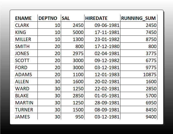
Q26. Running Sum: Write a query to calculate the running sum of salaries for employees in each department, ordered by hire date.
SELECT
    EMPNO, ENAME, DEPTNO, SAL, HIREDATE,
    SUM(SAL) OVER (PARTITION BY DEPTNO ORDER BY HIREDATE ROWS UNBOUNDED PRECEDING) AS running_sum
FROM EMP
ORDER BY DEPTNO, HIREDA
Q27. Top-N per Group: Retrieve the top 2 earners in each department along with their salaries.
WITH top_earners AS (
    SELECT
        EMPNO, ENAME, DEPTNO, SAL,
        DENSE_RANK() OVER (PARTITION BY DEPTNO ORDER BY SAL DESC) AS salary_rank
    FROM EMP
)
SELECT EMPNO, ENAME, DEPTNO, SAL
FROM top_earners
WHERE salary_rank <= 2
ORDER BY DEPTNO, salary_rank;
Q28. Second Last Hire: For each employee, find the date of their second-to-last hire using LEAD()/LAG().
WITH hire_order AS (
    SELECT
        EMPNO, ENAME, HIREDATE, DEPTNO,
        LAG(HIREDATE, 1) OVER (PARTITION BY DEPTNO ORDER BY HIREDATE DESC) AS second_last_hire
    FROM EMP
)
SELECT EMPNO, ENAME, DEPTNO, HIREDATE
FROM hire_order
WHERE second_last_hire IS NULL;
Q29. Compared to Nth Value: Show employees who earn more than the 2nd highest salary in their department.
WITH dept_ranked AS (
    SELECT
        EMPNO, ENAME, DEPTNO, SAL,
        DENSE_RANK() OVER (PARTITION BY DEPTNO ORDER BY SAL DESC) AS rank
    FROM EMP
),
second_highest AS (
    SELECT DEPTNO, SAL
    FROM dept_ranked
    WHERE rank = 2
)
SELECT e.EMPNO, e.ENAME, e.DEPTNO, e.SAL
FROM EMP e
JOIN second_highest s ON e.DEPTNO = s.DEPTNO
WHERE e.SAL > s.SAL;
Q30. Gaps in Sequences Detection: Identify missing invoice numbers in a table (e.g., 100, 101, 103, 104,107,110 → gap at 102, gap at 105-106, gap at 108-109).
Dataset –
100, ‘Alice Smith’, 150.00,
101, ‘Bob Johnson’, 200.00,
103, ‘Charlie Brown’, 175.50, — Gap: 102 is missing
104, ‘Diana Prince’, 300.00,
107, ‘Edward Norton’, 225.75, — Gaps: 105-106 missing
110, ‘Fiona Green’, 180.00 — Gaps: 108-109 missing
WITH numbered_invoices AS (
    SELECT
        invoice_num,
        LEAD(invoice_num) OVER (ORDER BY invoice_num) AS next_num
    FROM invoices
)
SELECT invoice_num + 1 AS gap_start,
       next_num - 1 AS gap_end
FROM numbered_invoices
WHERE next_num - invoice_num > 1;
- WITH numbered_invoices AS (
SELECT invoice_num, LEAD(invoice_num) OVER (ORDER BY invoice_num) AS next_num FROM invoices
)- This creates a temporary result set where each row contains:
invoice_num: The current invoice numbernext_num: The next invoice number in sequence (using LEAD())
- This creates a temporary result set where each row contains:
- Intermediate Results:
After the CTE executes, it would look like this:
invoice_num next_num
100 101
101 103
103 104
104 107
107 110
110 NULL - Main Query Logic:
SELECT invoice_num + 1 AS gap_start, next_num – 1 AS gap_end
FROM numbered_invoices
WHERE next_num – invoice_num > 1;
- For each row, it calculates:
gap_start: current invoice + 1 (first missing number)gap_end: next invoice – 1 (last missing number)
- The WHERE clause only includes rows where there’s a gap (>1 difference)
- For each row, it calculates:
- Final Output:
The query returns:
gap_start gap_end
102 102(Only 102 is missing between 101 and 103)
105 106(105 and 106 missing between 104 and 107)
108 109(108 and 109 missing between 107 and 110)
Q31. Consecutive Days: Find users who logged in for 3 or more consecutive days
WITH login_dates AS (
  SELECT
    user_id,
    login_date,
    LAG(login_date, 2) OVER (PARTITION BY user_id ORDER BY login_date) AS two_days_prior
  FROM user_logins
)
SELECT DISTINCT user_id
FROM login_dates
WHERE login_date = two_days_prior + INTERVAL '2 days';
Q32. Previous/Next Row Comparison: Compare each month’s sales to previous month
SELECT
  month,
  sales,
  LAG(sales, 1) OVER (ORDER BY month) AS prev_month_sales,
  sales - LAG(sales, 1) OVER (ORDER BY month) AS month_over_month_change,
  (sales - LAG(sales, 1) OVER (ORDER BY month)) / LAG(sales, 1) OVER (ORDER BY month) * 100 AS growth_percentage
FROM monthly_sales;
Q33. First and Last in Group: For each department, display the first and last hired employee’s name and hire date.
WITH department_employees AS (
  SELECT
    department_id,
    employee_name,
    hire_date,
    FIRST_VALUE(employee_name) OVER (PARTITION BY department_id ORDER BY hire_date) AS first_employee,
    FIRST_VALUE(hire_date) OVER (PARTITION BY department_id ORDER BY hire_date) AS first_hire_date,
    LAST_VALUE(employee_name) OVER (PARTITION BY department_id ORDER BY hire_date
      RANGE BETWEEN UNBOUNDED PRECEDING AND UNBOUNDED FOLLOWING) AS last_employee,
    LAST_VALUE(hire_date) OVER (PARTITION BY department_id ORDER BY hire_date
      RANGE BETWEEN UNBOUNDED PRECEDING AND UNBOUNDED FOLLOWING) AS last_hire_date,
    ROW_NUMBER() OVER (PARTITION BY department_id ORDER BY hire_date) AS rn
  FROM employees
)
SELECT
  department_id,
  first_employee,
  first_hire_date,
  last_employee,
  last_hire_date
FROM department_employees
WHERE rn = 1;
Q34. Cumulative Sum Reset: Running total of sales that resets each year
SELECT
  date,
  sales,
  SUM(sales) OVER (PARTITION BY EXTRACT(YEAR FROM date) ORDER BY date) AS yearly_running_total
FROM daily_sales;
Q35. Customer Retention: Identify customers who made a purchase in the current month but not in the previous month
WITH customer_monthly_activity AS (
  SELECT
    customer_id,
    DATE_TRUNC('month', order_date) AS month,
    LAG(DATE_TRUNC('month', order_date)) OVER (PARTITION BY customer_id ORDER BY DATE_TRUNC('month', order_date)) AS prev_month
  FROM orders
)
SELECT
  customer_id,
  month AS current_month
FROM customer_monthly_activity
WHERE DATE_TRUNC('month', month) = DATE_TRUNC('month', CURRENT_DATE)
  AND (prev_month IS NULL OR prev_month < month - INTERVAL '1 month');
Q36. Sessionization: Group user activity logs into sessions (if inactivity > 30 mins, start a new session)
WITH activity_with_gaps AS (
  SELECT
    user_id,
    activity_time,
    LAG(activity_time) OVER (PARTITION BY user_id ORDER BY activity_time) AS prev_activity_time,
    CASE
      WHEN EXTRACT(EPOCH FROM (activity_time - LAG(activity_time) OVER (PARTITION BY user_id ORDER BY activity_time))) / 60 > 30
      THEN 1
      ELSE 0
    END AS new_session_flag
  FROM user_activity
),
session_groups AS (
  SELECT
    user_id,
    activity_time,
    SUM(new_session_flag) OVER (PARTITION BY user_id ORDER BY activity_time) AS session_id
  FROM activity_with_gaps
)
SELECT
  user_id,
  session_id,
  MIN(activity_time) AS session_start,
  MAX(activity_time) AS session_end,
  COUNT(*) AS activities_in_session
FROM session_groups
GROUP BY user_id, session_id;
Q37. Pareto Analysis (80/20 Rule): Find the top 20% of customers contributing to 80% of sales
WITH customer_sales AS (
  SELECT
    customer_id,
    SUM(order_amount) AS total_sales,
    SUM(SUM(order_amount)) OVER () AS grand_total,
    ROW_NUMBER() OVER (ORDER BY SUM(order_amount) DESC) AS rank
  FROM orders
  GROUP BY customer_id
),
running_totals AS (
  SELECT
    customer_id,
    total_sales,
    SUM(total_sales) OVER (ORDER BY total_sales DESC) AS running_sum,
    grand_total,
    running_sum / grand_total AS running_percentage
  FROM customer_sales
)
SELECT
  customer_id,
  total_sales,
  running_percentage
FROM running_totals
WHERE running_percentage <= 0.8
ORDER BY total_sales DESC;
Q38. Time Between Events: Calculate the average time between orders for each customer
WITH order_times AS (
  SELECT
    customer_id,
    order_date,
    LEAD(order_date) OVER (PARTITION BY customer_id ORDER BY order_date) AS next_order_date
  FROM orders
),
time_differences AS (
  SELECT
    customer_id,
    EXTRACT(EPOCH FROM (next_order_date - order_date)) / 86400 AS days_between_orders
  FROM order_times
  WHERE next_order_date IS NOT NULL
)
SELECT
  customer_id,
  AVG(days_between_orders) AS avg_days_between_orders
FROM time_differences
GROUP BY customer_id;
Q39. Partitioned Running Count: For each product category, show a running count of orders by date
SELECT
  order_date,
  product_category,
  COUNT(*) AS daily_orders,
  SUM(COUNT(*)) OVER (PARTITION BY product_category ORDER BY order_date) AS running_category_orders
FROM orders
GROUP BY order_date, product_category
ORDER BY product_category, order_date;
Q40. Alternate Row Selection: Select every 2nd row from a result set
WITH numbered_rows AS (
  SELECT
    *,
    ROW_NUMBER() OVER (ORDER BY id) AS row_num
  FROM my_table
)
SELECT *
FROM numbered_rows
WHERE MOD(row_num, 2) = 0;
Q41. Deduplication: Remove duplicate rows (keeping one copy)
WITH duplicates AS (
  SELECT
    *,
    ROW_NUMBER() OVER (PARTITION BY column1, column2, column3 ORDER BY id) AS row_num
  FROM my_table
)
DELETE FROM my_table
WHERE id IN (
  SELECT id FROM duplicates WHERE row_num > 1
);
Q42. Hierarchical Running Sum: Compute a running total that respects a hierarchy (e.g., sum sales by region → country → city)
SELECT
  region,
  country,
  city,
  sales_date,
  sales_amount,
  SUM(sales_amount) OVER (PARTITION BY region, country, city ORDER BY sales_date) AS city_running_total,
  SUM(sales_amount) OVER (PARTITION BY region, country ORDER BY sales_date) AS country_running_total,
  SUM(sales_amount) OVER (PARTITION BY region ORDER BY sales_date) AS region_running_total
FROM sales_data
ORDER BY region, country, city, sales_date;
Q43. Conditional Running Sum: Calculate a running sum that only includes values meeting a condition (e.g., sum sales where amount > 100)
SELECT
  date,
  amount,
  SUM(CASE WHEN amount > 100 THEN amount ELSE 0 END)
    OVER (ORDER BY date) AS conditional_running_sum
FROM transactions;
Q44. Dynamic Window Sizes: Write a query where the window frame size varies by row (e.g., 7-day average for weekdays, 3-day for weekends)
SELECT
date, sales, CASE WHEN EXTRACT(DOW FROM date) BETWEEN 1 AND 5 THEN — Weekday
AVG(sales) OVER (ORDER BY date ROWS BETWEEN 3 PRECEDING AND 3 FOLLOWING)
ELSE — Weekend
AVG(sales) OVER (ORDER BY date ROWS BETWEEN 1 PRECEDING AND 1 FOLLOWING)
END AS dynamic_avg
FROM daily_sales;
If you’re looking to master window functions in Snowflake SQL, the Snowflake Window Functions Documentation provides an excellent reference guide