How Snowflake Uses Memory and Threads for Parallel Processing becomes clear when you examine what happens after a SQL statement is submitted. Snowflake query execution begins by parsing and validating the query, generating an optimized execution plan, and then running it on distributed compute resources. Inside a virtual warehouse, multiple execution threads work in parallel while sharing a common memory pool. Snowflake relies on cost-based optimization and dynamic task scheduling to distribute work efficiently across these threads. Parallel processing occurs as execution threads scan micro-partitions concurrently, and memory is dynamically allocated across operators such as scans, joins, and aggregations. This adaptive, shared-resource architecture enables Snowflake to deliver scalable performance without requiring manual tuning of memory or thread allocation.
1. How Does Snowflake Parse and Execute a SQL Query?
When you submit a SQL query in Snowflake, a lot happens before a single row is returned. It may feel instant, but internally there is a well-defined pipeline that converts your text into a fully distributed execution plan.
Let’s walk through the full lifecycle in a clear, structured way. I’ll use a simple example:
SELECT customer_id, SUM(amount)
FROM orders
WHERE order_date >= '2025-01-01'
GROUP BY customer_id;
We’ll trace what happens from the moment you hit Enter to the moment results come back.
High-Level Stages
When a query is submitted, Snowflake processes it in these main stages:
- Parsing
- Semantic analysis
- Logical plan generation
- Optimization
- Physical plan creation
- Execution planning and task scheduling
- Distributed execution
- Result construction and return
Now let’s go deeper into each stage.
1. Query Submission
When you execute SQL from:
- Snowsight
- SnowSQL
- JDBC/ODBC
- Python connector
The SQL text is sent to the Cloud Services layer, not directly to the warehouse.
Important separation:
- Cloud Services → parsing, optimization, metadata
- Virtual Warehouse → actual execution
2. Parsing (Syntax Analysis)
This is the first real processing step.
The parser checks:
- Is the SQL syntactically valid?
- Are keywords used correctly?
- Are parentheses balanced?
- Is the structure legal?
It does NOT yet check if tables exist.
The parser converts your SQL string into an internal structure called a:
👉 Abstract Syntax Tree (AST)
Think of it as a tree representation of the query.
For our example:
- SELECT
- columns: customer_id, SUM(amount)
- FROM
- table: orders
- WHERE
- condition: order_date >= ‘2025-01-01’
- GROUP BY
- customer_id
If there’s a syntax mistake, error happens here.
End result of parsing:
A structured tree representation of your SQL.
3. Semantic Analysis (Validation Stage)
Now Snowflake validates meaning.
It checks:
- Does
orderstable exist? - Does
customer_idexist in that table? - Is
amountnumeric (valid for SUM)? - Do you have access privileges?
- Does GROUP BY match selected columns?
It resolves:
- Fully qualified table names
- Column data types
- Schema references
- Role permissions
If table does not exist or you lack permission, error happens here.
End result:
A validated query structure with resolved metadata.
4. Logical Plan Generation
Now Snowflake converts the validated query into a logical plan.
Logical plan describes:
- What operations must happen
- In what order
- Independent of hardware
For our query, logical operations are:
- Scan orders
- Filter order_date >= ‘2025-01-01’
- Group by customer_id
- Compute SUM(amount)
This plan is still abstract.
It does not yet say:
- How many threads
- How many tasks
- Which CPU
- Memory layout
It only defines relational operations.
5. Query Optimization (Cost-Based Optimizer)
This is one of the most important stages.
Snowflake now decides the most efficient way to execute the query.
It uses:
- Table statistics
- Micro-partition metadata
- Data distribution
- Cardinality estimates
- Predicate selectivity
For example:
Micro-partition pruning
If only 10 percent of partitions contain order_date >= ‘2025-01-01’
Snowflake eliminates 90 percent before scanning.
This decision happens here.
Optimizer decisions include:
- Join order (if multiple tables)
- Filter pushdown
- Aggregation pushdown
- Partition pruning
- Choosing hash vs merge join
- Choosing broadcast vs distributed join
- Choosing parallel degree
End result:
An optimized logical execution plan.
6. Physical Plan Creation
Now Snowflake converts logical plan into a physical execution plan.
This stage determines:
- How many execution operators
- How data is distributed
- How tasks are split
- How many parallel threads
For example:
Instead of:
Scan → Filter → Aggregate
It becomes:
- Parallel scan operators
- Local aggregation nodes
- Exchange nodes (for data redistribution)
- Final aggregation node
This physical plan is what you see in:
👉 Query Profile
Operators like:
- TableScan
- Filter
- HashAggregate
- Exchange
- Sort
End result:
A distributed execution DAG (Directed Acyclic Graph).
7. Task Scheduling in Warehouse
Now Cloud Services sends execution plan to the Virtual Warehouse.
Warehouse:
- Allocates compute threads
- Splits work into execution tasks
- Distributes tasks across CPUs
Example:
If warehouse has 32 cores:
- 32 scan tasks may run in parallel
- Each task reads different micro-partitions
Tasks are created based on:
- Data size
- Partition count
- Operation type
- Available compute
This is where multithreading begins.
8. Distributed Execution
Now execution starts.
Step 1: Scan
Each thread reads assigned micro-partitions.
Step 2: Filter
Predicate applied locally inside each thread.
Step 3: Local Aggregation
Each thread computes partial SUM(amount) per customer_id.
Step 4: Exchange
Data is reshuffled if needed for final grouping.
Step 5: Final Aggregation
Global SUM per customer_id computed.
All this happens in parallel across CPUs.
9. Result Materialization
After final aggregation:
- Results are gathered
- Sorted if required
- Serialized into result set format
If result set is small:
Returned directly to client.
If large:
Stored temporarily in result storage.
Snowflake also caches results for:
👉 Result cache reuse (if identical query runs again)
What Is the Final End Result of Parsing?
If you strictly ask:
What does parsing produce?
Answer:
It produces a validated Abstract Syntax Tree (AST).
But practically, the end product of the whole compilation pipeline is:
👉 A fully optimized distributed physical execution plan ready for parallel execution.
That plan:
- Knows exactly which partitions to scan
- Knows how data flows between tasks
- Knows aggregation strategy
- Knows parallel degree
- Knows memory allocation strategy
Where You Can See This
You cannot see AST directly.
But you can see:
- Logical + physical plan in Query Profile
- Operator tree
- Execution graph
- Data volume between nodes
- Skew indicators
Complete Flow Summary
User SQL
→ Parser (syntax check)
→ Semantic Analyzer (object validation)
→ Logical Plan
→ Cost-Based Optimizer
→ Physical Plan
→ Task Scheduler
→ Parallel Execution
→ Result Materialization
→ Client receives rows
Key Architectural Insight
Snowflake separates:
Control Plane (Cloud Services):
- Parsing
- Optimization
- Metadata
- Planning
Data Plane (Warehouse):
- Execution
- Parallel processing
- Thread-level work
This separation allows:
- Better scaling
- Reusable planning
- Efficient execution
- Multi-cluster support
2. How Snowflake Uses Memory and Threads for Parallel Processing – A Practical Explanation
When you start learning Snowflake architecture, one of the first things you hear is that warehouse size determines compute power. You’ll see statements like: X-Small warehouse has 1 node. It has about 8 execution threads. It has roughly 16 GB of memory. At that point, it’s very natural to think in simple mathematical terms. If there are 8 threads and 16 GB of memory, then maybe each thread gets 2 GB. And if a micro-partition is roughly 16 MB compressed, you might calculate that 2 GB divided by 16 MB equals about 125 micro-partitions per thread. That sounds logical at first glance. But this is not how Snowflake actually works.
To understand how Snowflake Uses Memory and Threads for Parallel Processing, we need to step back and understand the architecture more clearly. A Snowflake warehouse consists of compute nodes. Each node contains CPU execution threads, memory, local SSD cache, and network bandwidth. However, memory is not statically divided among threads. Threads are units of CPU execution. Memory is a shared resource used dynamically by query operators. That difference is extremely important.
Let’s walk through a practical example. Assume you have a 10 GB compressed table. Since the average micro-partition size is around 16 MB compressed, that table would contain roughly 640 micro-partitions. Now suppose your query applies a filter that eliminates 75 percent of the partitions using micro-partition pruning. That leaves about 160 micro-partitions to scan. You are using an X-Small warehouse with approximately 8 execution threads.
Now here is the key point. Even though the warehouse has about 16 GB of memory and 8 threads, Snowflake does not assign 2 GB of memory to each thread. Memory is not sliced evenly and locked per thread. Instead, all operators running inside the node request memory dynamically from a shared pool. That memory is used for scan buffers, decompression buffers, hash tables for joins, aggregation maps, sorting buffers, result staging, and network exchange. Threads do not “own” memory. They borrow what they need and release it.
When Snowflake begins scanning the 160 micro-partitions, it creates a queue of scan tasks. Each micro-partition becomes a unit of work. At any given moment, only as many partitions can be processed in parallel as there are available execution threads. In an X-Small warehouse, that means roughly 8 partitions are processed simultaneously. Thread 1 takes the first partition. Thread 2 takes the second. This continues until all 8 threads are busy. As soon as one thread finishes processing its partition, it pulls the next available partition from the queue. This continues until all 160 partitions are processed. In this case, it would take roughly 20 waves of scheduling, but the scheduling is dynamic rather than rigid.
Inside each thread, processing is also more efficient than many people imagine. A thread does not load an entire 16 MB compressed micro-partition fully into memory and hold it there. Instead, Snowflake processes data in a streaming and vectorized manner. It reads only the required columns, decompresses column chunks in batches, applies filters to thousands of values at once using vectorized CPU instructions, emits qualifying rows, and reuses the memory buffers for the next chunk. Because of this streaming model, it is unnecessary and inefficient to load 125 micro-partitions into memory per thread even if memory capacity theoretically allows it. CPU concurrency, not memory division, determines true parallelism.
This is why the assumption “2 GB per thread means 125 partitions at once” does not reflect actual execution behavior. Even if memory were abundant, processing 125 partitions simultaneously on a single thread would not increase CPU parallelism. The thread can execute only one instruction stream at a time. Loading excessive partitions would only increase memory pressure and reduce cache efficiency without improving throughput.
To make the scaling pattern clearer, consider how warehouse sizes grow. Snowflake does not publish exact hardware specifications, but the scaling pattern is consistent and widely understood. An X-Small warehouse has 1 compute node with about 8 threads and roughly 16 GB of memory. A Small warehouse has 2 nodes with about 16 threads and around 32 GB of memory. A Medium warehouse has 4 nodes with roughly 32 threads and 64 GB of memory. A Large warehouse has 8 nodes with about 64 threads and around 128 GB of memory. Each size roughly doubles the compute nodes, doubles the threads, doubles memory, and increases I/O bandwidth proportionally. Parallelism increases because thread count increases, not because memory is divided more thinly.
So the correct mental model is this. Threads determine how many tasks can run at the same time. Micro-partitions determine how finely the work can be divided. Memory supports the execution engine dynamically. When you understand how Snowflake Uses Memory and Threads for Parallel Processing, you realize that concurrency comes from execution threads pulling independent micro-partitions from a work queue, while memory is shared and allocated based on operator demand. That design is what allows Snowflake to scale predictably, avoid skew issues, and process large datasets efficiently without requiring users to manually manage partitions or memory allocation.
Here is a simplified conceptual view of warehouse scaling. Snowflake does not publish exact hardware specifications, but the scaling pattern is consistent:
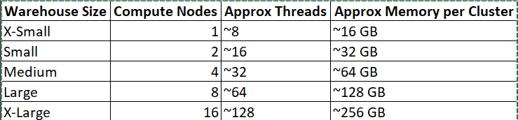
Each time you scale up, Snowflake roughly doubles compute nodes, CPU threads, memory, and I/O bandwidth. Parallelism increases because thread count increases, not because memory is divided differently.